Special Topics in Archaeology Final Project

For our final project in GIS5999, we were encouraged to come up with our own project and use many of the tools we've learned over the last year.  

For many decades the first colonizers of the Americas were a group of people called the Clovis tradition.  This has been challenged in recent years by sites that are as old or older than known Clovis sites.  Recently, the Western Stemmed Tradition culture (refers to a style of lithic point) has been found to be as old or older than Clovis.  I was able to acquire the database of WST points for the Oregon Burns District of the Bureau of Land Management.  I've worked at a site in this district for the last couple summers and thought it would be interesting to expand upon this work.  Map 1 shows the distribution of known WST artifacts across the Burns District.

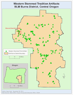
Map 1

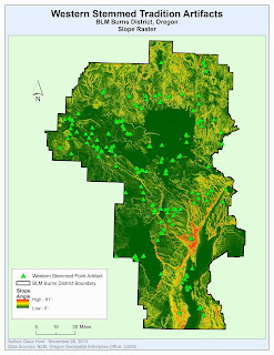
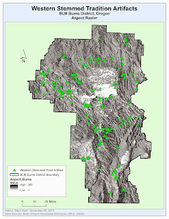
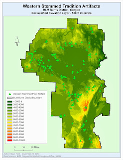
My project involves creating a predictive model.  A predictive model should help archaeologists plan future surveys by highlighting areas that are likely to produce more sites and save time by avoiding areas with low probability of producing sites.  My model will use proximity to water, elevation, slope, and aspect (direction towards the sun) to produce the predictive model.  Map 2 shows all the water features (lakes and streams) in the district with a 200 meter exterior buffer. Map 3 shows the elevation model for the district.  Map 4 is a slope raster produced from the DEM.  And, Map 5 is an aspect raster also produced from the DEM.

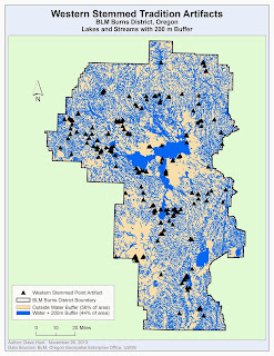
Map 2

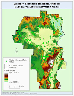
Map 3

Map 4

Map 5

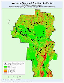
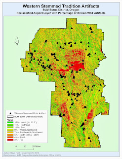
For this predictive model, I had the advantage of having the database of locations for 414 known WST artifacts.  Using this information, I was able to use an ArcMap tool (Extract Values to Points) to determine how artifacts were grouped within each component.  For example, for elevation, I created a layer divided into intervals of 500 feet each (i.e., 4000 - 4500, 4500 - 5000, etc.). Then, using the Extract Values to Points tool, I could determine how many artifacts fell into which interval. From this information, I could determine the percentage of artifacts in each class and Reclassify the raster to hold that value.  Map 6 is the water buffer map reclassified to show that 63% of artifacts occur within 200m of water while 37% of artifacts occur outside that buffer.  Map 7 is the reclassified elevation map, showing that most WST artifacts occur between 4000 and 5500 feet.  Map 8 is the reclassified slope map, showing that most WST artifacts occur on flatter terrain.  Map 9 is the reclassified slope map showing that, surprisingly, most WST artifacts occur in a Northerly aspect.

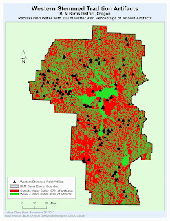
Map 6

Map 7

Map 8

Map 9

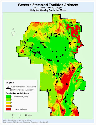
The Weighted Overlay tool in ArcMap allows us to assign relative values then to each of these rasters and combine them, based on that value and the reclassified values within them, into a single "weighted" raster.  This combination should provide a whole, more useful than its parts, that can be used to determine which areas are more likely to yield further WST sites.  Map 10 is the final weighted overlay from this analysis. Green areas a good areas to conduct further survey research, red are likely poor areas.  

Map 10

Overall, I was a little disappointed with the generalized look of this predictive model.  In the future, I would like to refine it and hopefully tighten up the areas that are most highly weighted. 

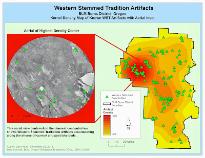
In addition to the weighted overlay, I was curious about producing a density map based on known WST artifacts.  This is shown in Map 11.  This map also includes an aerial image of the center of the densest region.  Looking at the aerial, we can see that, in fact, many of the artifacts in this densest region are on the shores of dry lakes.  One area that might help tighten the predictive model is to just use the lakes features and exclude streams.  Streams (and 200m buffers around them) consume an enormous area of the map and perhaps WST people were more inclined to live along lake shores than stream banks.  This is an area I will research further.

Map 11

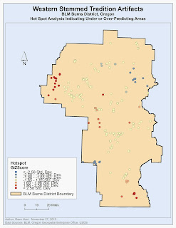
Finally, for the graduate student requirement, we conducted some statistical tests on our results.  Map 12 shows the result of a Hot Spot analysis following an Ordinary Least Squares analysis.  The red dots indicate areas where more WST artifacts are occurring than would be expected.  I found it encouraging that my field work is occurring near the red dots in the western-most portion of Map 12.

Map 12

Overall this was a pretty intense final lab.  It was a lot of work, but I think the results are useful or will be useful with some further refining.  I am optimistic that we may find some interesting patterns regarding where Western Stemmed Tradition people congregated on the landscape and this may be useful as part of the pursuit for determining who was first in the Americas.

Biscayne Bay Shipwrecks - Weighted Overlay

This week we continued with our project focused on Biscayne Bay shipwrecks. We began by creating 300 meter buffers around our 5 known shipwrecks to help us understand the benthic bottom types (for example consolidated sediments vs. reef terraces).  These various bottom types are shown in the map above.

The second map takes the benthic bottom and bathymetric layers we created last week and converted them to reclassified layers.  For the benthic bottom types, we grouped various bottom types into 5 classes that have increasing likelihood of shipwrecks (this from external known data).  For the bathymetric layer, we used natural breaks to create 5 groups representing the depths of the areas.  These two reclassified layers are shows above.

The final step was combining these two reclassified layers into one layer.  In doing this, we also wanted to weight one layer more highly than the other (70% benthic bottom type, 30% bathymetric). In doing this, we're saying that we think the benthic bottom type is a better indicator of where shipwrecks might occur.  The final product is the map above, with areas in red indicating areas that we may want to survey in the future to locate more shipwrecks.

Supervised Classification

Supervised Classification using Bands 4, 5, and 6

The final regular season lab for Remote Sensing was a supervised classification of a developing city (Germantown in Maryland).  We began with an aerial image of the town along with coordinates for 12 known land cover types.  After locating these points in the image, I used the technique of growing spectral signatures from a seed.  This involves setting a Spectral Euclidean Distance (mostly an estimate at first) and letting ERDAS Imagine build a polygon of pixels starting at the point you designate and emanating out to the spectral distance you selected.  This produces very interesting results and it is both fun and useful to play a bit with the distance to get the best signature of the known terrain.

Once the signatures are complete, it is important to verify that there is no spectral confusion (overlap) between signatures.  I found the widest separation in the signatures was found in Bands 4, 5, and 6, so I used these bands to create the supervised image.  I also merged the like signatures (we had multiple signatures for the same land cover, like "agriculture") into single classifications. Creating a set of classes also allows one to estimate the area dedicated i the image to each class.  The final supervised classification is presented above.

Biscayne Bay Shipwrecks - Part 1

This week begins with the first of a three-part lab involving GIS and shipwrecks!  I am super excited about this lab as this is exactly the reason I signed up for the GIS Certificate program at UWF in the first place.  The first part of this lab is about collecting the data we'll need for later stages of the lab.  We were provided a modern-day nautical chart (left) of Biscayne Bay National Park and the locations of five shipwrecks along the Maritime Heritage Trail (an underwater trail!).  We then had to locate an historical map (center) and the bathymetry data (right, in the form of a digital elevation model) for the park. From this maps, we get a sense of the conditions that led to these ships coming to grief in this particular part of the Florida Keys.

Unsupervised Classification

Unsupervised Classification of the UWF Campus

This week in Remote Sensing we used an aerial image of the UWF campus to try some unsupervised classification techniques.  Unsupervised classification is when we rely on the computer to group like pixels together and make assumptions that these represent similar features.  In the image above, we started by using ERDAS Imagine tools to create 50 unsupervised classes.  Then I manually assigned these 50 classes to 5 categories (Buildings/Roads, Trees, Grass, Shadows, and Mixed).  This process actually is pretty easy and goes quickly with the ERDAS tools.  This was one of the first assignments where I felt like the ERDAS tools were easier to use for this task than a similar task in ArcMap.  From the 5 new classifications, I was able to create an estimate of the permeable versus impermeable surfaces that make up the UWF campus.

GIS Internship - Article Review

Review of Mapping Benthic Habitats; the Marine GIS Challenge by Joe Breman

ArcUser Online, Spring 2005

http://www.esri.com/news/arcnews/spring05articles/mapping-benthic.html 

In Mapping Benthic Habitats; the Marine GIS Challenge, the author offers an outline of the challenges of both modeling the ocean floor and then making important conservation decisions with that model.  I chose this topic as it covers several areas of interest to me personally.  I am a recent UWF Maritime Studies graduate, so I have a strong interest in the ocean and all things maritime.  I am also a current UWF GIS Certificate student and this topic covers the use of various GIS tool in the process of mapping the ocean floor.   Finally, I am an avid SCUBA diver and have a strong interest in conservation of ocean resources and wildlife and the end result of this study is a better understanding of the areas we need to conserve.

The article primarily discusses two types of GIS tools.  The author notes that there is an extensive database of benthic sensor data.  We have been taking sonar readings and scans of many parts of the US coast for decades and this provides a rich set of data to be utilized.  Most of the data is simple x, y, and z point data and is easily converted to surfaces using tools readily available in ArcMap such as  the Inverse Distance Weighting, Spline or Terrain Dataset tools.  Once the surface is created, 3D Analyst can be used to visualize the ocean floor and assign a “bottom type” to each cell in the model.  These types are then used in mapping out habitat regions that need to be conserved for different species.  Making this process all the more complicated is that some species spend different portions of their lives (i.e., juvenile and adult) in differing habitat types.

Overall the report was informative, albeit rather brief.  I am especially interested in 3D modeling and wish that we had an entire separate class on it as part of the GIS Certificate.  I would like to continue on in my own studies and expand my skill set using 3D modeling.  I am also glad to see GIS tools being used effectively for conservation and, hopefully, improving or minimizing our human impact on some of these areas that are often “out of sight, out of mind” for most of the general public.

Scythian Mounds, Final Report

The final lab for the Scythian mounds project involved creating the final predictive results based on our previous work.

Using these surfaces, we created a feature class of random points (minimum 30 m spacing) throughout the study area and merged these points with the possible mounds identified from an aerial image.  This feature class was then expanded with fields and filled with the values from the reclassified surfaces (elevation, aspect, and slope).  These points were then subjected to an Ordinary Least Squares linear regression method based on these three surfaces (top map above).

The results of the OLS give the following results:

               Adjusted R-Squared:   0.760202

	Coefficient	Probability
Intercept	-1.770434	0.000000
Aspect	0.115368	0.000001
Slope	0.113834	0.000001
Elevation	0.630913	0.000000

The Adjusted R-Squared value of 0.760 suggests that the three surface variables can explain 76.0% of the sites in the predictive model.

Since the coefficient values are positive (with the exception of Intercept) and not very close to zero, it appears that each surface property is making a positive contributing to the model results (with our reclassified weightings).  The probability values < 0.05 also support this conclusion (near 100% confidence level for each coefficient).

We also subjected our OLS results to a spatial autocorrelation test, returning the following results:

z-score: 11.43385

p-value: 0

The very low (zero) p value indicates that it is very unlikely that the data is distributed randomly.  The high Z-score (in conjunction with the low p value) indicates that the data is normally distributed and spatially autocorrelated.

Based on a visual review of the OLS residuals and hot spot analysis, it does appear that many of the predicted areas are within valley bottoms.  It may be beneficial to add an additional variable that accounts for this spatial distribution, such as access to water in the form of rivers and streams.

It does appear that we have established that the variables in use are helpful for use in a predictive model. Per the lab, it would probably be a good idea to test these variables further with a larger point set and additional regression models (such as GWR).  Additionally the variables should be analyzed further to ensure the relationships are truly linear.  Adding additional variables (such as access to water) may also expose additional relationships.  Finally, any model should be subjected to some ground truthing to understand if it is truly useful.