Final Project

Our final project for GIS 5990 was a substantial research project.  I chose to continue with the Valley of Oaxaca data that we had used in the Digitization module.  An important anthropological question is whether there is a relationship between population intensity, limitations on the carrying capacity of the land, and a resultant emergence of government. One way to study this relationship is with “site catchment analysis” (Vita-Finzi and Higgs 1970:5) which can be used to determine whether the carrying capacity (the ability of the land to produce food) is exceeded in later cultural phases as populations expand.

The project involved determining the site catchment buffer for the archaeological sites in several 4km square grids within the valley.  In the image above, I've created 1 km buffers around the Phase IIIA site for my grids.  The sites have been converted to points, allowing me to create Thiessen polygons around each point.  Thiessen polygons allow us to divide up an area so that each point on the map is within a region closest to one of the site points.  This helps prevent double counting of territory.

With the catchment buffer established, and with the help of land cover shapefiles we had built earlier, I was able to determine how many hectares of each type of land/soil were within the catchment area for each site.  This could then be used, along with some information from the literature about corn cob lengths during the various phases and resultant crop yields, to determine the number of metric tons of corn grown around each site.  Assuming that a family of five could live on a metric ton of maize for a year, we can estimate the highest possible population supported by the catchment buffer.

In the end, my results showed that the catchment return was quite high and that agricultural limitations do not appear to factor into either settlement patterns nor provide support for the emergence of government in later cultural phases within the Valley of Oaxaca.

Remote Sensing

This week's assignment focused on using remote sensing resources and raster classification (both unsupervised and supervised) methods in an attempt to locate unknown archaeological sites.  Our first attempt (above) was an "unsupervised" classification of land cover by the ArcGIS program.  Unsupervised means that the program basically tried to divide the region up into classes (we asked for 8 classes) based on the coloration of our aerial (which was gray-scale).  This led to a lot of errors and redundancy.  Specifically, water bodies (which seem to be quite green) and forest areas were frequently confused. In the same way, the mounds at Cahokia Mounds State Park, and specifically Monk's Mound, were classified along with field grass and roads and buildings.

In the second part of the assignment, we created a point shapefile and selected land cover around the map.  I added over 60 points and manually classified them as water, forest, fields, roads, buildings and mounds. Unfortunately, the results of this "supervised" classification were not much better than the unsupervised.  There was still a lot of redundancy and errors in areas with similar color (water/forests) and some areas (like residential areas) were classified as a mix of water and forest rather than building sites.  It was interesting to try these methods, but I'm doubtful on whether they can be effective for archaeological work.

Finally, the grads played around with chi-square tests.  This test is super useful and I've used it in classes in the past.  The key seems to be finding or setting up data in a way that allows the use of this test.  That is a tool that I want to be ready and able to use when analyzing field results.

Surface Interpolations

 

This module was quite challenging and involved the creation of 14 different "maps" (for grad students) that are combined into a sort of poster for demonstrating the power of surface interpolation.  I found these exercises to be extremely practical as I am personally focusing on landscape archaeology and these sorts of statistical exercises and surface interpolations seem certain to factor into my future work.

The first set of maps demonstrates different density and surface interpolation examples on the same set of shovel test data (total artifacts) created by Dr. Palumbo in Panama.  I preferred the result from Kernel Density (with a radius of 50) as it seemed the most straightforward result.  The interpolation surfaces (Kriging, IDW, Spline, and Natural Neighbor) use various mathematical models to create predictive surfaces.

The second poster focuses on data converted from AutoCAD for the Machalilla region.  This was a useful exercise in understanding how to convert common data types to ArcGIS and then manipulate it by using tables and joins.  One complicating factor was that the AutoCAD data has no coordinate system.  The data appears to be in kilometers (probably former 17S UTM data set to a local datum). This allowed me to create a scale bar in kilometers.  We also used the largest polygon in the conversion as the study area boundary and this was used for clipping the rasters.  For reasons inexplicable, I had one clip exhibit "the donut effect" (kernel density) but the other clips do not.

Finally, the grads continued with the Machalilla data to create a series of Inverse Distance Weighting interpolations set to differing powers in an attempt to replicate the Peterson & Drennan (2005) article. The general idea is that social interaction occurs within communities (in this case, in the Regional Development Period) and that clusters occur across the landscape with a (subjective) distance (perhaps of < 2 km) acting as the limiting factor of daily communication between these community clusters. By applying an IDW with various weightings, we can find the smoothing point where community clusters reach this interaction limit and gain some understanding of how communities were manifest on the landscape.  The power of 1 seemed to provide a good view that didn't have too much "steepness" or intensity while also smoothing out to about 2 km clusters.  This seems to show intense community interaction in the southeast corner of the region that seems to sweep in a curve west and north to and up the coast.  These seems to be an isolated region in the middle of this area of interconnectedness.

Finally, the grads worked some stats problems using the t-test.  I liked the Drennan (1996) reading so much, I bought his book.

Digitizing Archaeological Maps and Data

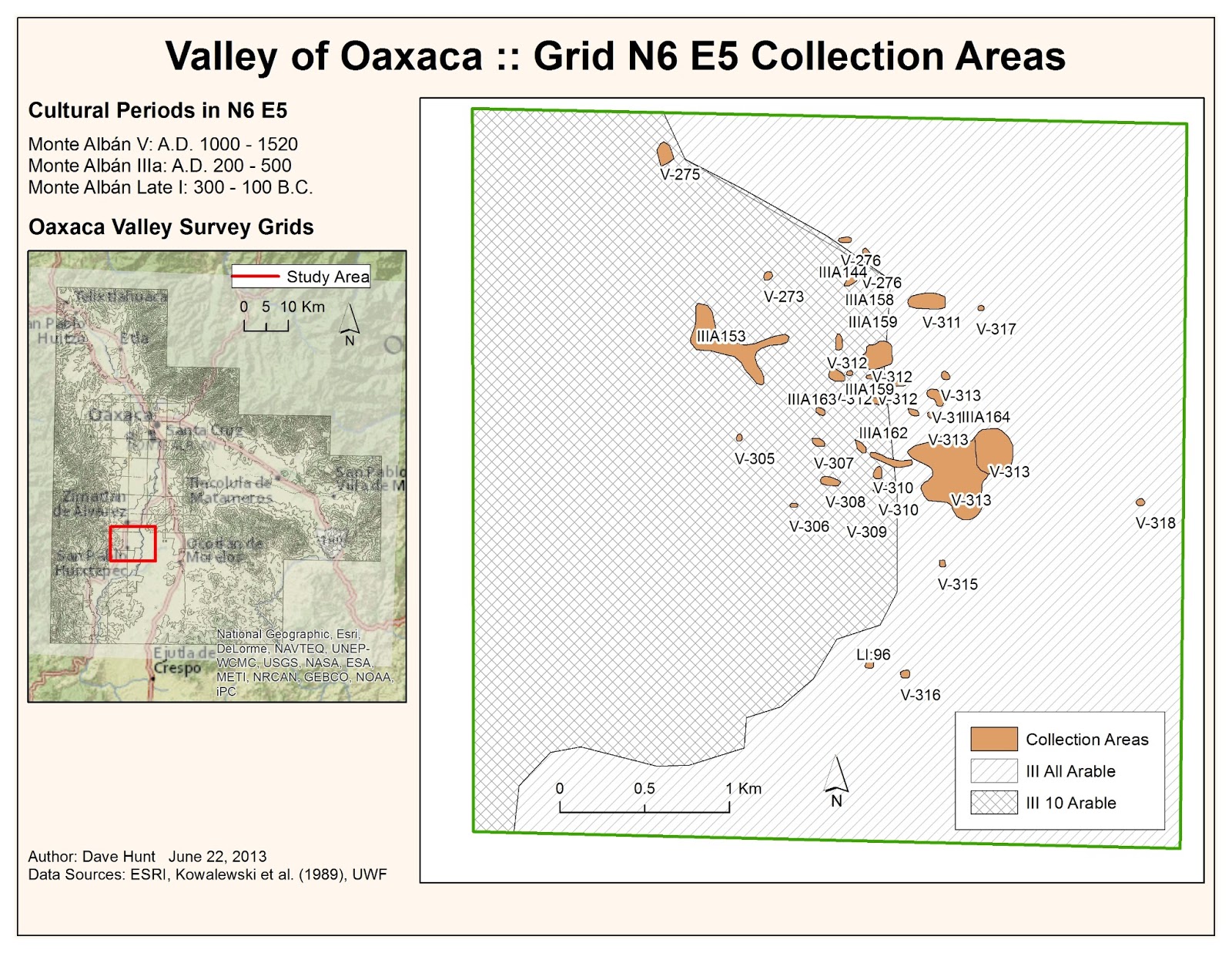
This week's assignment was pretty interesting and one that should be pretty useful for anyone working in a region that has had a lot of fieldwork in previous decades, specifically prior to computerization of records.  The general idea was using older documents from a Valley of Oaxaca (Mexico) survey, digitizing and geoprocessing those maps onto an ArcGIS basemap, digitizing various aspects of the maps (sites and land use) and then using data from the original surveys to do analysis.  The first map (above) shows my three assigned grid (N6 E4, N6 E5, and N6 E6) geoprocessed onto a digital topographic map and also the larger Valley of Oaxaca survey area.

The biggest challenge was getting the larger survey map geoprocessed onto the base map.  My original base map selection contained far too many political objects and the topographic features were hard to see and match up with the survey area scan.  I did find a base map that seemed to have fewer objects cluttering the topography although it would be nice to fine a base map that was just topographical without towns, roads, etc.  Once the main survey scan was in place, it was relatively simple matter to geolocate the assigned grids.  The corners matched up quickly and easily and there seemed to be good correspondence, particularly with the soil type maps.

The second part of the lab involved creating an individual map for each of our assigned grids (below). For these maps, we digitized the site collection areas as polygons and captured the cultural period data from field notes.

The biggest challenge was initially understanding the original drawings.  However, once I entered “field note-taker” mode, it was pretty easy to understand how they were labeling each collection area.  Creating the collection area polygons progressed fairly quickly though there were some annoyances with polygons closing themselves too early and the stop/edit attribute table/delete bad polygon/start editing again process.  I used label classes to deal with the multiple cultural periods per collection area.  Some areas are quite crowded and therefore clutters.  Overall, I was pretty happy with the end result.

Finally, the grad students continued on to join some additional site data to the existing digitized collections for a specific cultural period.  I didn’t have any IIIB artifacts in my three assigned grids, so I used IIIA (of which I had a lot) to demonstrate the join to the additional data table.  The join was quite straightforward and after segregating IIIA collection polygons to their own layer, I simply adjusted the symbology to use the joined lopop field and appropriately color grade the sites based on their estimated low populations.

Georeferencing - Macao Then and Now

This week's assignment was pretty interesting and involved georeferencing historical maps to contemporary maps.  The light yellow map above is a map of Macao (China) produced by Captain Cook (and William Bligh) in 1775.  This map was obviously created at a time both latitude and especially longitude were difficult to determine with high accuracy.  To "fit" this map to a modern map, we use Control Points to match landmarks that appear to be unchanged over the time between the two maps.  A lot has gone on in Macao since 1775.  In particular, there appears to be a lot of land reclamation that filled in areas between the islands of Macao.  To find control points, it was especially useful to look at a topographical map and look for the landmarks that would have stood out to sailors mapping from a ship. In a few places (particularly to the north) we see a great deal of distortion. This is either the result of inaccurate distances in the original map or mismatch on my part. However, most of the smaller islands seem to be in about the right place.

This was a pretty fun assignment and one that will be super useful for anyone doing historic archaeology.

Historical Archaeology

This week in Archaeological Applications, we focused on online sources of historical data and the lab specifically focused on the retrieval and use of historical maps and documents. There are numerous sources for materials that archaeologists may need.  Our lab took us to Ancestry.com, Arcgis.com, and Google Maps Street View. From a technical perspective, we also explored including hyperlinks within a map.

Graphical design and layout is probably one of my weaknesses when it comes to maps, so more practice is good, I suppose.  I do always feel like I'm cramming more items into a map than could possibly fit however.

Ethics and Archaeology

This week in GIS Applications in Archaeology we focused on ethics. Each major archaeological society has a statement regarding ethics and the important role that archaeologists need to take in protecting archaeological sites and discouraging the trade in artifacts.  The graduate reading also discussed the use of tools like Google Earth to monitor important archaeological sites for looting.  The primary example focused on the country of Jordan. We also each provided a summary of our view on ethics in archaeology, a discussion that will, no doubt, get pretty interesting.

To follow that up, we explored the MEGA Jordan site and created a feature class based on the coordinates retrieved from this site. The premier site in Jordan is, of course, Petra, as any Indiana Jones fan and archaeologist should know.  These sites are presented in the map above.

On the practical side, the exercise involved using a file geodatabase as the repository for our "sensitive" data.  The file geodatabase is a good choice for archaeologists as it easy to move (just zip up the folder), has few size limits (limited only by disk space) and can be easily secured (save to removable drive or encrypt the folder). The easier it is to secure information about precious sites, the less likely it will fall into the hands of those who what to exploit it.

The Great Chicago Fire

This first assignment for GIS Applications in Archaeology explored some historical data from before and after Chicago's Great Fire of 1871.  In this assignment, we looked at historical buildings built prior to 1871 and how they were affected by the fire.  We could see that none were actually built in the fire zone.  However, after the fire (which burned 4 square miles of the city) we see a large number of buildings popping up in what must have been a largely vacant area of the city.  Also interesting to note is that we can tell the directly of the wind during the fire as origin point is known.  We can clearly see the fire being blown northeast by a wind from the southwest until the fire runs into the shore of Lake Michigan.

Technically, this was largely a review week, as all the tools and processes were ones that we covered in the first semester. Still, I am very excited about this class. It will be great to focus specifically on the use of GIS tools for archaeology.